Guide to the Avellaneda & Stoikov Strategy

Avellaneda & Stoikov 전략 가이드

Hummingbot 아카데미에 다시 오신 것을 환영합니다!

최신 Hummingbot 릴리스(0.38)에서는 고전적인 학술적 마켓 메이킹 모델에 기반한 흥미로운 전략을 선보입니다. 이 글에서는 2008년의 Avellaneda & Stoikov 논문과 Hummingbot에서의 구현에 대해 자세히 알아보겠습니다.

심도 있는 과학 논문을 즐기시는 분들을 위해, 원본 논문은 온라인이나 여기에서 직접 찾아보실 수 있습니다.

오늘 우리가 살펴볼 내용은 다음과 같습니다:

• Avellaneda & Stoikov 마켓 메이킹 모델
• 재고 위험 관리
• 최적의 매수 및 매도 스프레드 결정
• Hummingbot에서의 구현

1️⃣ Avellaneda & Stoikov 모델 이해하기

이 모델은 마켓 메이커의 두 가지 주요 관심사를 다룹니다:

• 재고 위험 관리
• 최적의 매수 및 매도 스프레드 결정

Avellaneda & Stoikov는 마켓 메이커가 이러한 문제를 해결하는 데 도움이 되는 공식을 제안합니다.

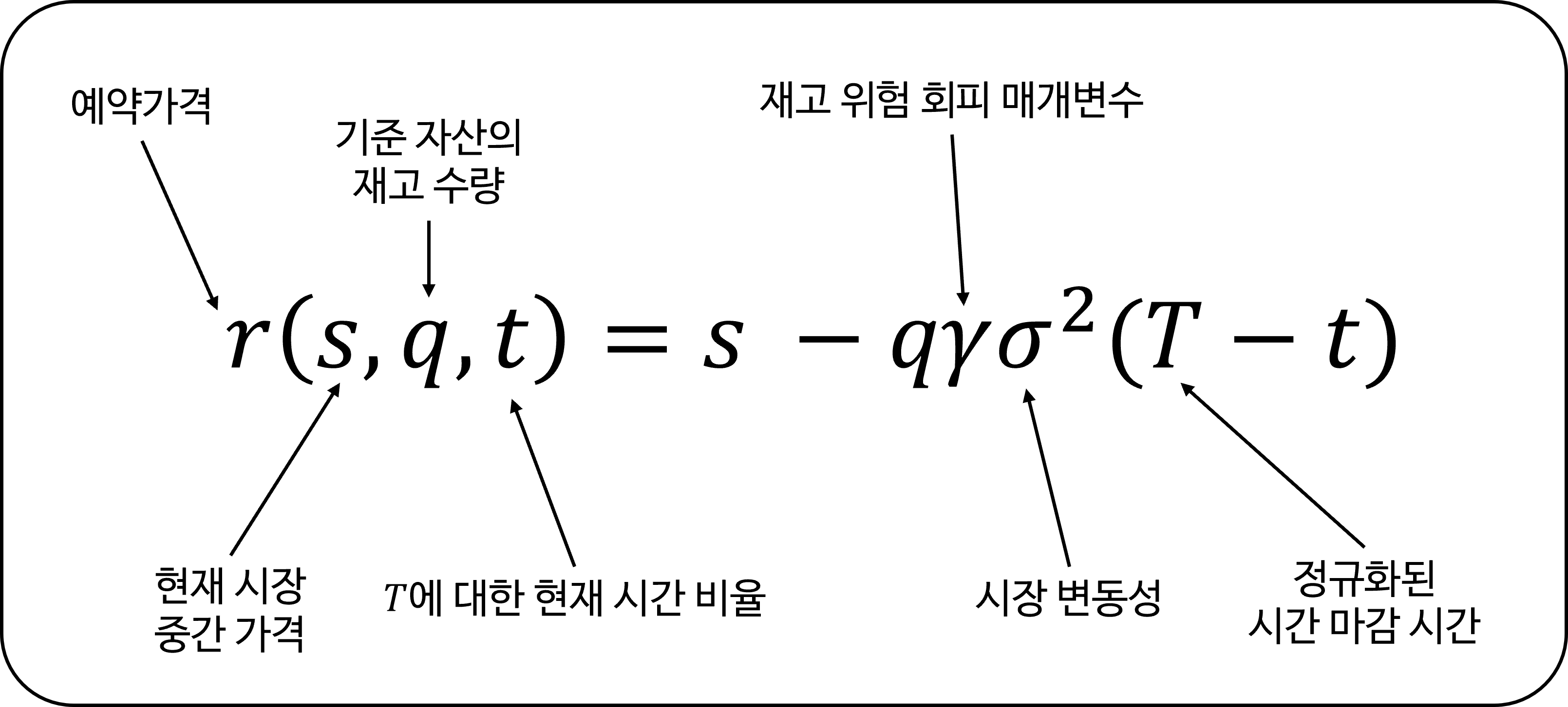
예약 가격 (Reservation price):

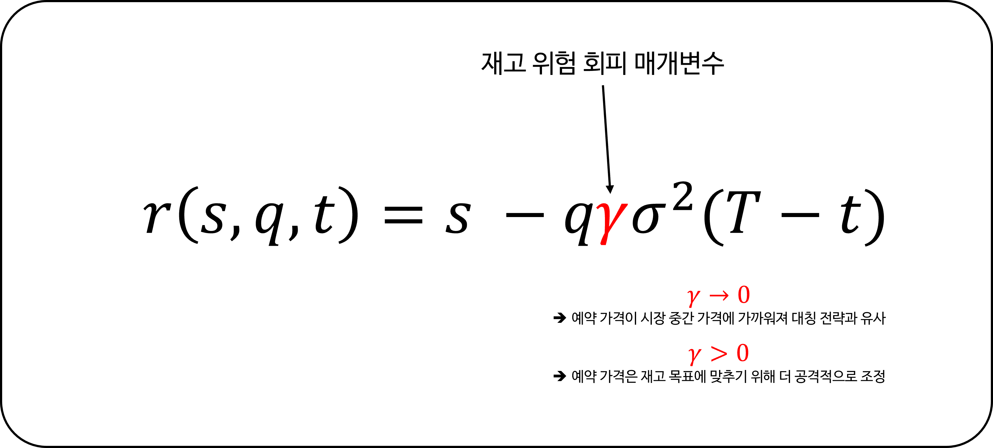
\[r(s, q, t) = s - q \gamma \sigma^2 (T - t)\]

최적 매수 및 매도 스프레드 (Optimal bid & ask spread):

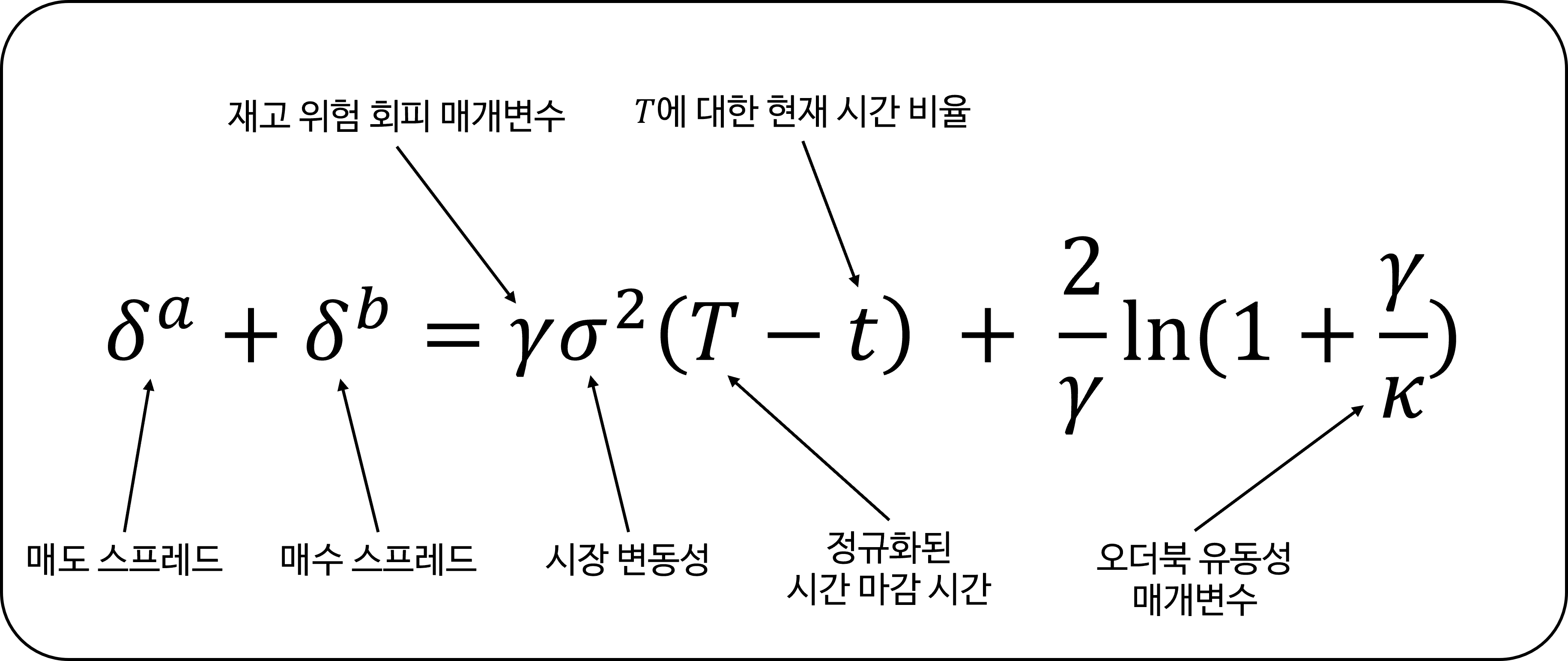
\[\delta^a + \delta^b = \gamma \sigma^2 (T - t) + \frac{2}{\gamma}\ln \left(1 + \frac{\gamma}{\kappa}\right)\]

여기서 각 변수는 다음을 의미합니다:

• $s$ = 현재 시장 중간 가격
• $q$ = 기준 자산의 재고 수량 (롱/숏 포지션에 따라 양수/음수)
• $\sigma$ = 시장 변동성
• $T$ = 정규화된 마감 시간 (1)
• $t$ = $T$에 대한 현재 시간의 비율
• $\delta^a, \delta^b$ = 대칭적인 매수/매도 스프레드
• $\gamma$ = 재고 위험 회피 매개변수
• $\kappa$ = 오더북 유동성 매개변수

이 글에서는 이러한 공식과 그 의미를 간단하게 설명합니다. 더 기술적인 세부 사항을 다루는 후속 기사를 기대해 주세요.

2️⃣ 예약 가격 설명

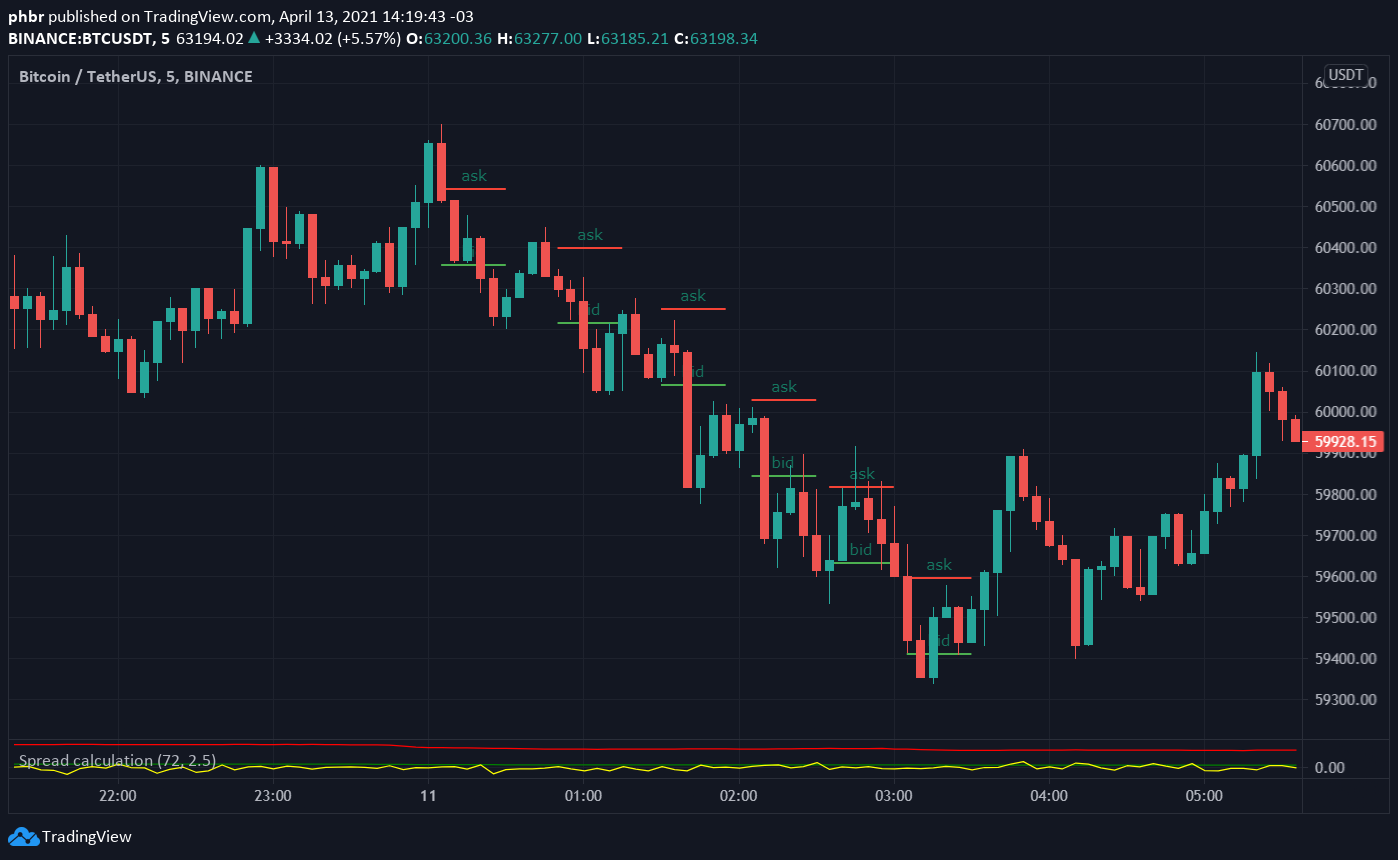
전통적인 마켓 메이킹은 시장 중간 가격을 중심으로 대칭적인(symmetrical) 매수 및 매도 주문을 내는 것을 포함합니다. 하지만 이는 재고 편향으로 이어질 수 있으며, 자산 가치가 불리하게 움직일 경우 트레이더를 위험에 빠뜨릴 수 있습니다.

예를 들어, BTC-USDT 하락 추세에서 대칭 전략을 사용하면 마켓 메이커는 결국 BTC를 축적하게 되어 총 재고 가치가 감소합니다.

Avellaneda & Stoikov의 접근 방식은 다음을 고려하여 주문 배치를 위한 새로운 기준 가격을 계산합니다:

\[r(s, q, t) = s - q \gamma \sigma^2 (T - t)\]

재고 포지션 편차 ($q$)

How distant is the trader’s current inventory position is from the target position?

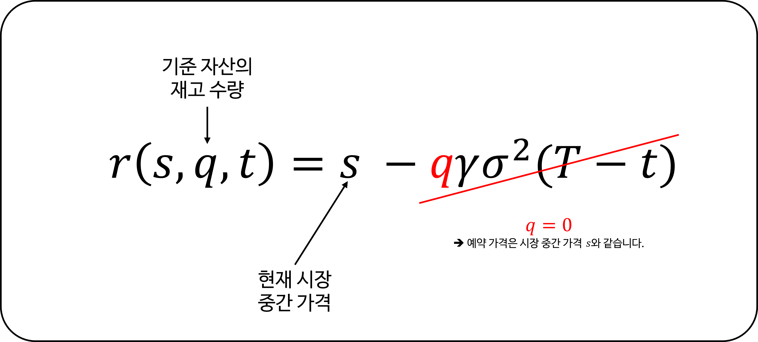
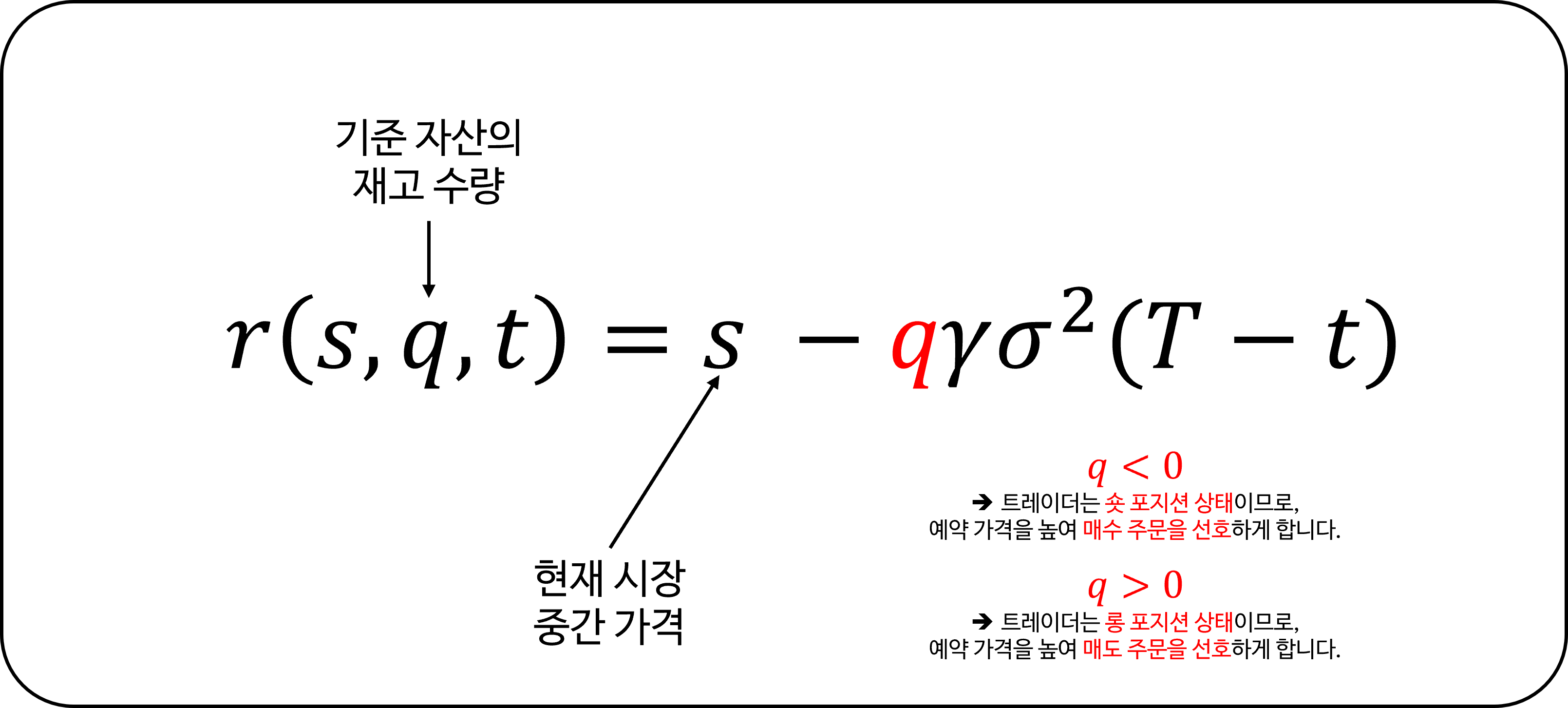
공식에서 $q$의 값은 목표 재고로부터의 편차를 나타냅니다. 예를 들어:

• $q = 0$일 때, 예약 가격은 시장 중간 가격과 같습니다.
• $q < 0$일 때, 트레이더는 숏 포지션 상태이므로, 예약 가격을 높여 매수 주문을 선호하게 합니다.
• $q > 0$일 때, 트레이더는 롱 포지션 상태이므로, 예약 가격을 낮춰 매도 주문을 선호하게 합니다.

Hummingbot은 사용자가 지정한 목표 재고 비율을 기반으로 $q$를 계산합니다.

재고 위험 감수도 ($\gamma$)

How much inventory risk does the trader want to take?

트레이더가 설정하는 이 매개변수는 재고 위험을 감수하려는 의지를 나타냅니다. $\gamma$가 0에 가까우면 예약 가격이 시장 중간 가격에 가까워져 대칭 전략과 유사해집니다. $\gamma$가 증가하면 예약 가격은 재고 목표에 맞추기 위해 더 공격적으로 조정됩니다.

Hummingbot에서는 $\gamma$를 수동으로 설정하거나 자동으로 계산할 수 있습니다.

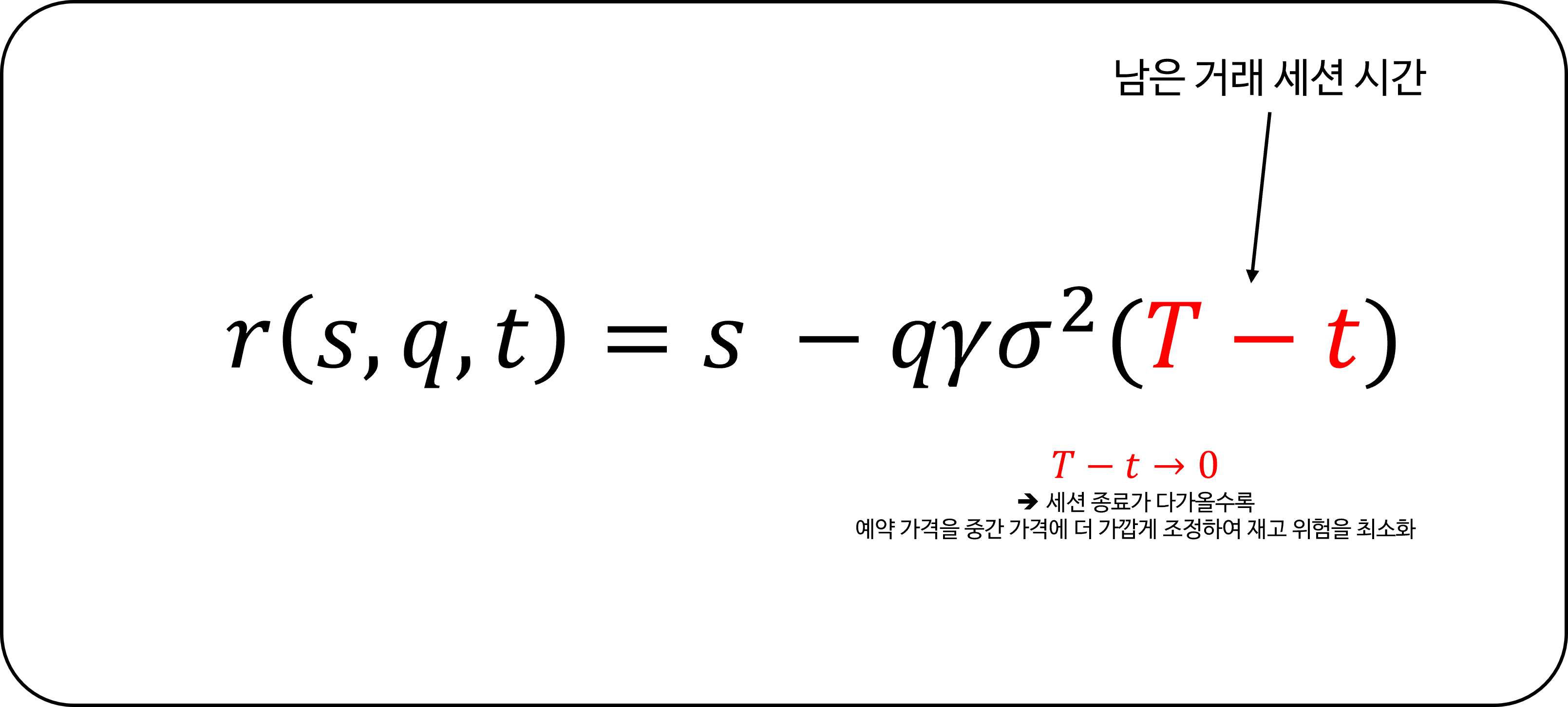
남은 거래 세션 시간 ($T-t$)

Time until the trading session ends

거래 세션이 정해진 전통적인 금융 시장을 고려하여, 이 모델은 세션 종료가 다가올수록 예약 가격을 중간 가격에 더 가깝게 조정하여 재고 위험을 최소화합니다.

Hummingbot에서는 거래 세션 기간을 설정하여 24/7 운영되는 암호화폐 시장에 맞게 모델을 조정할 수 있습니다.

참고: Avellaneda & Stoikov는 연속적인 시장에 더 적합한 무한 시간 모델(infinite horizon model)도 제안했으며, 이는 향후 릴리스에 포함될 계획입니다.

시장 변동성($\sigma$)

시장 변동성($\sigma$) 또한 예약 가격에 영향을 미치지만 트레이더가 정의하는 요소는 아닙니다. 변동성이 증가하면 예약 가격과 중간 가격 사이의 격차가 넓어집니다.

3️⃣ 최적 스프레드 결정하기

모델의 두 번째 측면은 수익성을 위한 최적의 오더북 포지셔닝에 중점을 둡니다.

\[\delta^a + \delta^b = \gamma \sigma^2 (T - t) + \frac{2}{\gamma}\ln\left(1+\frac{\gamma}{\kappa}\right)\]

여기서는 예약 가격의 요소$\gamma$와 $T-t$가 다시 등장하며, 추가적으로 다음이 포함됩니다:

오더북 유동성 ($\kappa$)

논문에서는 수학적 세부 사항을 깊이 다루지만, 핵심은 높은 $\kappa$ 값이 더 촘촘한 오더북을 의미하며 더 작은 스프레드가 필요하다는 것입니다. 반대로, 낮은 $\kappa$는 유동성이 적음을 시사하므로 더 넓은 스프레드를 허용합니다.

4️⃣ 예약 가격과 최적 스프레드 결합하기

모델의 실행 로직은 간단합니다:

1. 목표 재고를 기반으로 예약 가격을 계산합니다.
2. 최적의 매수 및 매도 스프레드를 결정합니다.
3. 예약 가격을 중심으로 시장가 주문을 냅니다:
   • 매수 가격 = 예약 가격 - 최적 스프레드의 절반
   • 매도 가격 = 예약 가격 + 최적 스프레드의 절반

이러한 동적인 움직임은 아래에 설명되어 있습니다:

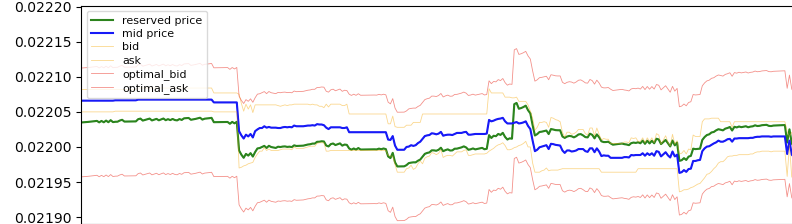
계산된 예약 가격(녹색 선)은 종종 시장 중간 가격(파란색 선)과 다릅니다. 예약 가격은 재고에 따라 조정되며, 중간 가격 대비 주문 배치에 영향을 미칩니다.

5️⃣ 매개변수 계산

Avellaneda-Stoikov 모델의 핵심 요소는 다음과 같습니다:

1. 재고 포지션 ($q$)
2. 남은 거래 세션 시간 ($T-t$)
3. 위험 계수 ($\gamma$)
4. 오더북 뎁스 ($\kappa$)

각각에 해당하는 Hummingbot 매개변수는 다음과 같습니다:

1. 재고 거리 ($q$): 현재 재고와 목표 재고 간의 차이를 반영합니다. Hummingbot에서 자산 재고 목표 비율을 설정하면 봇이 $q$를 계산합니다.
2. 세션 시간 ($T-t$): 멈추지 않는 암호화폐 시장의 특성에 맞게 모델을 조정합니다. Hummingbot에서 원하는 거래 세션 기간을 정의합니다.
3. 위험 계수 ($\gamma$) 및 오더북 뎁스 ($\kappa$): 논문에서는 이들의 계산법을 명시하지 않았지만, Hummingbot의 “이지 모드”는 원하는 스프레드 한도를 기반으로 자동으로 결정합니다. 또는 parameters_based_on_spread를 False로 설정하고 order_book_depth_factor와 risk_factor를 사용하여 수동으로 값을 입력할 수 있습니다.

6️⃣ Hummingbot 설정하기

Hummingbot에서 전략을 생성하려면 create 명령어를 사용하고 전략 이름으로 avellaneda_market_making을 지정해야 합니다.

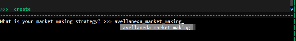
거래소와 거래 페어를 선택한 후, Hummingbot이 위험 계수와 오더북 뎁스를 계산하도록 할지 결정합니다.

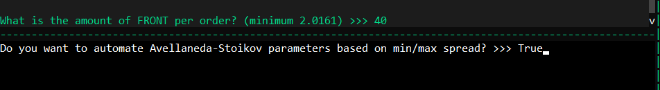
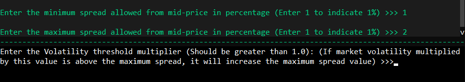
원하는 최대 및 최소 스프레드를 설정하여 계산된 최적 스프레드의 한도를 정의합니다.

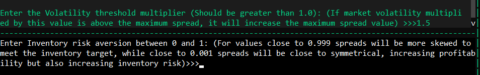
위험 회피 매개변수는 재고 위험 선호도를 결정합니다. 1에 가까운 값은 보수적인 접근 방식을 나타냅니다.

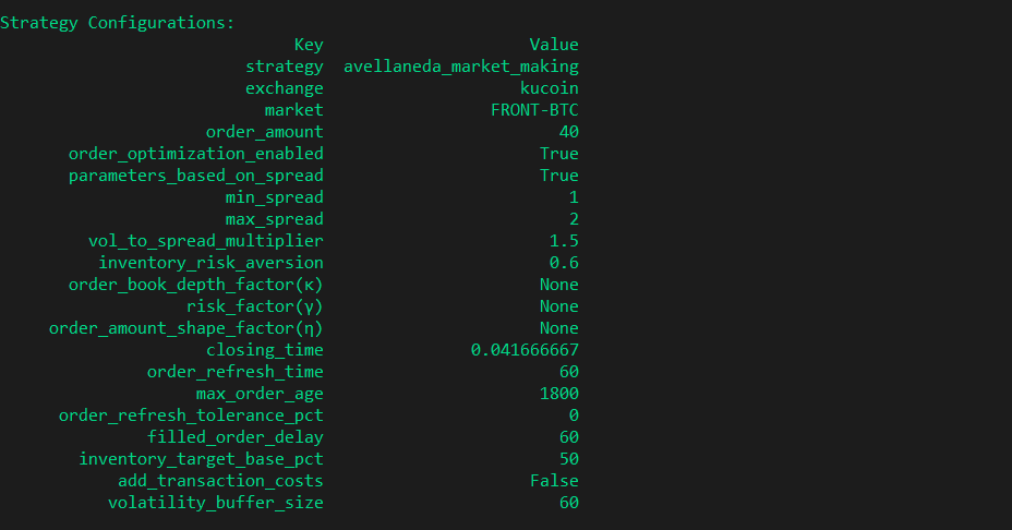
마지막으로, 총 재고 중 기준 자산이 차지해야 할 비율을 결정하는 재고 목표 비율을 지정합니다.

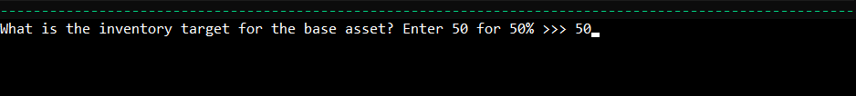
Hummingbot의 추가 설정에는 closing_time(세션 기간)과 volatility_buffer_size(변동성 계산을 위한 데이터 기간)가 포함됩니다.

7️⃣ 마지막 생각

최적의 마켓 메이킹 전략은 수십 년 동안 학술 연구의 초점이었습니다. 오늘날 시장에서 고빈도 매매(High-Frequency Trading, HFT)가 중요한 역할을 하는 만큼, 우리 팀이 탐구할 것이 많습니다. 제안할 흥미로운 모델이 있다면, 디스코드에서 저희와 함께하세요!

8️⃣ 커뮤니티에 참여하세요

저희 디스코드 채널에 참여하여 동료 마켓 메이커 및 차익거래자들과 교류하세요. 트위터와 레딧에서 저희를 팔로우하여 업데이트와 소식을 받아보세요. 저희 유튜브 채널에서 전문 트레이더와의 인터뷰를 포함한 마켓 메이킹에 대한 콘텐츠를 놓치지 마세요.

Show original (English)

# Guide to the Avellaneda & Stoikov Strategy  Welcome back to the Hummingbot Academy! The latest Hummingbot release (0.38) introduces an exciting strategy based on classical academic market-making models. This article will delve into the Avellaneda & Stoikov paper from 2008 and its implementation in Hummingbot. For those who enjoy in-depth scientific papers, the original publication is readily accessible online or directly [here](https://www.researchgate.net/publication/24086205_High_Frequency_Trading_in_a_Limit_Order_Book). Today we will explore: - The Avellaneda & Stoikov market-making model - Inventory risk management - Optimal bid & ask spread determination - Implementation in Hummingbot ## Understanding the Avellaneda & Stoikov Model The model addresses two primary concerns of market makers: * Inventory risk management * Optimal bid and ask spread determination Avellaneda & Stoikov propose formulas aiding market makers in addressing these challenges. Reservation price: $$ r(s, q, t) = s - q \gamma \sigma^2 (T - t) $$ Optimal bid & ask spread: $$ \delta^a + \delta^b = \gamma \sigma^2 (T - t) + \frac{2}{\gamma}\ln \left(1 + \frac{\gamma}{\kappa}\right) $$ Where, - $s$ = current market mid-price - $q$ = inventory quantity of base asset (positive/negative for long/short positions) - $\sigma$ = market volatility - $T$ = normalized closing time (1) - $t$ = current time as a fraction of \(T\) - $\delta^a$, $\delta^b$ = symmetrical bid/ask spread - $\gamma$ = inventory risk aversion parameter - $\kappa$ = order book liquidity parameter This article simplifies these formulas and their meanings. Stay tuned for an upcoming article with more technical details. ## Reservation Price Explained Traditional market making involves symmetrical bid and ask orders around the market's mid-price. However, this can lead to inventory skewing, potentially putting the trader at risk if the asset value moves unfavorably. For example, in a BTC-USDT downtrend using a symmetrical strategy, the market maker ends up accumulating BTC, decreasing the total inventory value.  Avellaneda & Stoikov's approach calculates a new reference price for order placement, considering: $$ r(s, q, t) = s - q \gamma \sigma^2 (T - t) $$ ### Inventory Position Deviation ($q$) The value of q in the formula represents the deviation from the target inventory. For example: * At $q = 0$, the reservation price equals the market mid-price; * At $q < 0$, the trader is short, raising the reservation price to favor buy orders; * At $q > 0$, the trader is long, lowering the reservation price to favor sell orders. Hummingbot calculates $q$ based on your specified target inventory percentage. ### Inventory Risk Tolerance ($\gamma$) This parameter, set by the trader, indicates willingness to take inventory risk. A near-zero $\gamma$ means the reservation price is close to the market mid-price, similar to a symmetrical strategy. As $\gamma$ increases, the reservation price adjusts more aggressively to match inventory targets. In Hummingbot, $\gamma$ can be manually set or automatically calculated. ### Remaining Trading Session Time ($T-t$) Considering traditional financial markets with defined trading sessions, this model adjusts the reservation price closer to the mid-price as the session end approaches, minimizing inventory risk. Hummingbot allows setting the trading session duration, adapting the model for 24/7 cryptocurrency markets. Note: Avellaneda & Stoikov also propose an infinite horizon model, more suitable for continuous markets, which we plan to include in future releases. Market volatility ($\sigma$) also influences the reservation price but is not a trader-defined factor. Increased volatility widens the gap between the reservation and mid-prices. ## Determining the Optimal Spread The model's second aspect focuses on the optimal order book positioning for profitability. $$ \delta^a | \delta^b = \gamma \sigma^2 (T - t) + \frac{2}{\gamma}ln(1+\frac{\gamma}{\kappa}) $$ Here, the reservation price factors ($\gamma$ and $(T-t)$) reappear, with the addition of: ### Order Book Liquidity ($\kappa$) While the paper delves into mathematical details, the key takeaway is that a high $\kappa$ value indicates denser order books, requiring smaller spreads. Conversely, a low $\kappa$ suggests less liquidity, allowing for wider spreads. ## Combining Reservation Price and Optimal Spread The model's execution logic is straightforward: 1. Calculate the reservation price based on target inventory. 2. Determine the optimal bid and ask spread. 3. Place market orders around the reservation price: - Bid price = reservation price - half of optimal spread - Ask price = reservation price + half of optimal spread This dynamic is illustrated below:  The calculated reservation price (green line) often deviates from the market mid-price (blue line). The reservation price adjusts based on inventory, influencing order placement relative to the mid-price. ## Parameter Calculations The key factors in the Avellaneda-Stoikov model are: 1. Inventory position ($q$) 2. Remaining trading session time ($T-t$) 3. Risk factor ($\gamma$) 4. Order book depth ($\kappa$) For each, the associated Hummingbot parameter is: 1. Inventory Distance ($q$): Reflects the difference between current and target inventory. In Hummingbot, set your asset inventory target percentage, and the bot calculates $q$. 2. Session Time ($T-t$): Adapts the model for the non-stop nature of cryptocurrency markets. Define your desired trading session duration in Hummingbot. 3. Risk Factor ($\gamma$) & Order Book Depth ($\kappa$): While the paper doesn't specify calculations for these, Hummingbot's "easy mode" automatically determines them based on desired spread limits. Alternatively, set config parameters_based_on_spread to False and manually input values using config order_book_depth_factor and config risk_factor. ## Configuring Hummingbot Creating the strategy in Hummingbot involves the create command and specifying avellaneda_market_making as the strategy name.  After selecting the exchange and trading pair, decide whether to let Hummingbot calculate the risk factor and order book depth.  Set your maximum and minimum desired spreads, which define the limits for the calculated optimal spread.  The risk aversion parameter dictates your inventory risk preference. A value close to 1 indicates a conservative approach.  Finally, specify your inventory target percentage, determining how much of your total inventory should be in the base asset.  Additional configurations in Hummingbot include closing_time (session duration) and volatility_buffer_size (data timeframe for volatility calculation).  ## Final Thoughts Optimal market-making strategies have been a focus of academic research for decades. With high-frequency trading (HFT) playing a significant role in today's markets, there's much for our team to explore. If you have an intriguing model to suggest, join us on Discord! ## Join Our Community Join our Discord channel to engage with fellow market makers and arbitrageurs. Follow us on Twitter and Reddit for updates and news. Don't miss our content on market making, including interviews with professional traders, on our Youtube Channel.

참고자료

• https://hummingbot.org/strategies/avellaneda-market-making
• https://hummingbot.org/blog/guide-to-the-avellaneda–stoikov-strategy/
• A comprehensive guide to Avellaneda & Stoikov’s market-making strategy
• High-frequency trading in a limit order book